

 The Boston Globe
Abstract
The 287(g) program enables local law enforcement agencies to enforce federal immigration laws. We examine 287(g)’s implementation across multiple counties in North Carolina and identify its impact on local crime rates and police clearance rates using a staggered difference-in-differences research design. Under multiple empirical specifications, we find no evidence to suggest that 287(g) programs had an effect on crime rates in North Carolina counties following their implementation. These results hold for simple measures of program adoption and program intensity. Our findings suggest that 287(g) in North Carolina counties did not meet its intended objective of improving public safety by facilitating the removal of violent offenders. Keywords: 287(g) Program, Interior Immigration Enforcement JEL Classification Numbers: K14, K37, K42, J18
1. Introduction
There is a common public perception that immigrants commit more crimes than native-born Americans. However, the empirical evidence near-uniformly finds that immigrants are either less or, at worst, equally as likely to be incarcerated or to commit crimes as natives (Green, 2016; Mears, 2001). Nevertheless, Congress created federal immigration enforcement programs to cooperate with local and state police to assist in the identification and removal of illegal immigrants (Kandel, 2016). How these immigration enforcement efforts impact violent and property crime rates is essential to judging whether they are worthwhile expenditures of scarce law enforcement resources, but there is little research on how local immigration enforcement programs affect crime rates (Miles & Cox, 2014).
We investigate how the federal immigration program 287(g) affected violent and property crimes rates in the state of North Carolina by estimating the elasticity of immigrant removals through the 287(g) program to county index crime rates. 287(g) is one of the most notorious immigration enforcement programs. It is named after Section 287(g) of the Immigration and Nationality Act that permits the Department of Homeland Security (DHS) to delegate immigration enforcement powers to state and local governments and to train their local law enforcement agencies (LEAs) in the investigation, apprehension, and detention of those suspected of violating immigration laws (Kandel, 2016). Local police officers with 287(g) training have access to federal immigration databases, can hold illegal immigrants for deportation, and produce court appearance documents for deportation proceedings (Kandel, 2016). By September 2012, 64 jurisdictions nationwide participated in 287(g) task force agreements that allowed police to arrest people solely on suspicion that they violated federal immigration law (Kandel, 2016; Outten-Mills, 2012).
In order to participate in 287(g) programs, local jurisdictions must sign a memorandum of agreement (MOA) with DHS that sets the parameters of cooperation (ICE, n.d.-a). There are three different types of 287(g) MOAs. The first are 287(g) jail enforcement agreements that allow local police to enforce federal immigration laws in jails and prisons by screening and identifying inmates who can be deported. The second are 287(g) task force agreements that deputize police officers to arrest illegal immigrants upon contact (Kandel, 2016). The third are hybrid 287(g) MOAs that combine both jail and task force agreements. In all three agreements, the LEA bears virtually all of the costs of enforcing 287(g) MOAs. In some cases, 287(g) LEAs either left the program or their MOAs expired.
This paper considers whether county adoption of 287(g) programs, measured by both the activation of 287(g) programs and the relative intensity of 287(g) enforcement, impacted violent and property crime rates in those North Carolina counties. To test a proposed linkage between the 287(g) program and crime rates, we use a staggered difference-in-differences research design that examines the effects of 287(g), measured by both program activation and intensity, on county crime rates. Our results are robust to a series of stringent robustness tests and show no evidence to suggest that 287(g) programs had a significant impact on crime in North Carolina. Furthermore, we find no evidence for geographic spillover effects in crime from 287(g) counties into non-287(g) counties.
2 Background
2.1 The 287(g) Program
Congress created the 287(g) program, which is named after Section 287(g) of the Immigration and Nationality Act, in 1996 as part of the Illegal Immigration Reform and Immigrant Responsibility Act (IIRIRA). 287(g) permits local, county, and state LEAs to sign a memorandum of agreement (MOA) with DHS which authorizes local authorities to enforce federal immigration law. At its peak, the 287(g) program had 71 signed MOAs in over 25 states.1Pedroza (2019) finds through FOIA records that between 2005-2012, DHS received 145 applications from local law enforcement agencies. Among these agencies, Dee and Murphy (2019) find that only around a third of these jurisdictions actually entered into 287(g) agreements. Dee and Murphy (2019) further note that available information from an application denial cites resource constraints as a cause for denial. Participation in the program itself is voluntary and local LEAs must first submit an application for consideration under 287(g). Upon acceptance into the program, select local law enforcement officers are deputized by DHS to perform the duties of federal immigration agents, including the arrest and processing of unauthorized immigrants for deportation during the course of routine police work. The federal government also monitors how LEAs enforce immigration laws to guarantee that they comply with the terms of the MOA.
There are three types of 287(g) agreement types: jail enforcement, task force, and hybrid models. The most common 287(g) MOAs are jail enforcement agreements, whereby specially trained officers within state and local correctional facilities identify criminal aliens in their custody through interviews and comparisons of their biometric information against the integrated DHS Automated Biometric Identification System (IDENT) and FBI Integrated Automated Fingerprint Identification System (IAFIS) databases (combined, IDENT/IAFIS). Although 287(g) corrections operations are restricted to jails on paper, counties were able to subvert these restrictions. We will describe that subversion later on. The second form of 287(g) agreement is the task force model, which allows ICE-deputized officers to conduct immigration-related investigations in the field. As mentioned, these two forms of 287(g) agreements could exist simultaneously as so-called hybrid models, which allowed local law enforcement to conduct immigration enforcement in a variety of settings, ranging from conducting citizenship status investigations during routine traffic stops or within correctional facility walls.
2.2 Coincidence with Secure Communities
One additional immigration enforcement program overlapped with 287(g) agreements in North Carolina — the Secure Communities program. Secure Communities is a universal and automated screening system that uses existing criminal background checks to immediately identify illegal immigrants for deportation using information from the IDENT/IAFIS biometric database. If the arrested individual’s fingerprints are flagged by DHS as likely belonging to an illegal immigrant then the federal government issues a “detainer request” or “ICE hold” that requests the local LEA to hold him for 48 hours beyond their scheduled release so that ICE can take custody for deportation. This also includes arrested illegal immigrants who were not charged with or convicted of crimes.
The federal government intended to roll out Secure Communities on a county-by-county basis beginning in October of 2008 along the US-Mexico border counties (Cox & Miles, 2013; ICE, 2009; Miles & Cox, 2014). About 97 percent of counties participated in Secure Communities by the Fall 2012 (Rosenblum & Kandel, 2013). Once enrolled, counties could not back out of the program or otherwise diminish their participation except by refusing to fingerprint arrestees, an option that no police departments exercised (Cox & Posner, 2012). President Barack Obama suspended Secure Communities in November 2014 (ICE, n.d.-b).
A key difference between the 287(g) program and Secure Communities is the disposition of removals. Under Secure Communities, arrestees’ fingerprints and biometric information were submitted to the federal government as part of an automated process, meaning that enforcement through Secure Communities would simply track the natural flow of arrestees into the system, ceteris paribus (Rugh & Hall, 2016).
3 North Carolina and 287(g)
To isolate how the 287(g) program affected crime, we focus on its implementation in the state of North Carolina as previous studies did.2See Nguyen and Gill (2010) and Nguyen and Gill (2016). Focusing on North Carolina provides numerous advantages over looking at other states or the nation as a whole for two reasons: empirical concerns of simultaneity between other programs in other states and the nature of 287(g) program implementation among North Carolina counties.
Not every 287(g) program was implemented in the same way. Stana (2009) found significant disparities in program implementation across 29 surveyed agencies due to limited guidance and oversight from ICE. A specific example of this took place in Alamance County, North Carolina, in which state troopers requested assistance from the Alamance County Sheriff ’s 287(g) deputies who were trained in corrections operations after pulling over a bus destined for Mexico (United States Cong. House. Committee on Homeland Security, 2009). Despite being deputized officially under a corrections MOA, 287(g) sheriff ’s deputies conducted immigration-related enforcement activities and summoned ICE agents to arrest five of the passengers (United States Cong. House. Committee on Homeland Security, 2009).
The second type of 287(g) MOA is a task force agreement that allows deputized local law enforcement officers to question and arrest illegal immigrants because of a suspected violation of federal immigration law (Kandel, 2016). In late 2012, President Barack Obama ordered all 287(g) task force agreements to expire at the end of that year while the jail enforcement agreements would continue (Kandel, 2016). State governments can also sign MOAs for state-wide police to participate in 287(g), but they are not very active compared to local LEAs. Local LEAs that participate in 287(g) are responsible for more than 15 times as many arrests of illegal immigrants that lead to deportation than states that also participate in the program. A full 93.9 percent of those deported under 287(g) task force agreements were arrested by local LEAs while state-wide police agencies are responsible for a mere 6.1 percent of all illegal immigrants removed under this program (ICE, 2010).
According to ICE, the 287(g) program’s intent was “to increase the safety and security of our communities by apprehending and removing undocumented criminal aliens who are involved in violent and serious crimes” (United States Cong. House. Committee on Homeland Security, 2009). This objective of crime reduction is echoed by Jim Pendergraph, the sheriff of Mecklenburg County, NC. He describes his office’s participation in 287(g) as a response to “the lack of [Congressional] action on the illegal immigration issue for decades, leaving those of us responsible for local law enforcement to deal with not only the fall-out of the criminal element, but the ire of the public for their perception of our inaction on a Federal issue” (United States Cong. House. Committee on Government Reform, Subcommittee on Criminal Justice, Drug Policy, and Human Resources, 2006). Similarly, Gaston County sheriff Alan Cloninger notes the aim of his office’s enrollment in 287(g) was “for the protection of the citizens of Gaston County” (United States Cong. House. Committee on Government Reform, Subcommittee on Criminal Justice, Drug Policy, and Human Resources, 2006).
Despite this designation of 287(g) as a crime-prevention mechanism by North Carolina sheriffs, 287(g) programs in North Carolina targeted nonviolent offenders and likely engaged in racial profiling. A study by the North Carolina ACLU in 2009 examined arrest data in Alamance and Mecklenburg Counties and found that local enforcement disproportionately targeted individuals for traffic violations based on race and nationality (Weissman, Deborah M and Headen, Rebecca C. and Parker, Katherine Lewis, 2009). Ultimately, the Department of Justice filed a lawsuit against the Alamance County sheriff for engaging in discriminatory policing against Hispanics (United States v. Johnson, 2012). Evidence of such practices indicate a divergence between stated ICE and local LEA goals for the program and their implementation at the local level. In the specific case of the lawsuit against the Alamance County Sheriff ’s Office, the court ruled in favor of the Sheriff ’s Office. Further investigation into the 287(g) program by Nguyen and Gill (2010) found that additional LEAs operating 287(g) programs in North Carolina showed a similar pattern of divergence from federal objectives and found no association between 287(g) enforcement and crime rates.
North Carolina presents an ideal target to empirically evaluate the anti-crime intent of the 287(g) program for a variety of reasons. For one, we avoid cross-contamination from other coexisting state and federal immigration enforcement activities, such as border enforcement and state-level enforcement laws such as Arizona’s SB 1070. Second, North Carolina counties represent a good cross-section of the United States, split almost evenly between metropolitan and rural areas.
4 Existing Literature
There is a sparse empirical literature examining the effects of 287(g) programs on various economic outcomes. Miles and Cox (2014) find that 287(g) activation lowers index crime rates by around 3 percent. Hines and Peri (2019) consider 287(g) program activation as a control to evaluate the crime effects of Secure Communities. Contrary to Miles and Cox (2014), they find no significant correlation between 287(g) adoption and changes in county crime rates, after controlling for deportations. While both of these studies incorporate 287(g) as a control variable, neither considers 287(g) as a primary independent variable. This paper fills this gap in the literature.
A more common examination in the literature pertains to 287(g) program effects on economic outcomes. One particular strand examines the potential labor market effects of deporting workers through 287(g). Kostandini, Mykerezi, and Escalante (2013) examine county-level data to identify the impact of 287(g) on the U.S. agricultural sector. They find that counties’ adoption of 287(g) agreements reduced local immigrant populations, leading to labor supply shocks within local agricultural markets and ensuing declines in agricultural wages and farm profits.3A later working paper from Ifft and Jodlowski (2016) finds a similar decline in farm profitability associated with participation in 287(g) agreements. They further find evidence for long-run implications in profitability related to 287(g) enforcement. There is also evidence that labor market effects induced by 287(g) enforcement go beyond the agricultural sector. Pham and Van (2010) find that 287(g) enforcement leads to overall declines in county employment levels. Bohn and Santillano (2017) further examine how 287(g) enforcement affects private employment, focusing in on immigrant-intensive industry sectors. Similarly, they find evidence for 287(g) labor supply shocks, primarily impacting administrative services employment. Rugh and Hall (2016) examine housing foreclosures and the degree to which deportations under 287(g) impacted foreclosure rates for Hispanic households. They consider the mechanism that deportation through programs such as 287(g) remove primary earners from households, thereby increasing rates of foreclosure. Using an inverse probability weighting strategy, their findings indicate that foreclosure rates among Hispanics increase in 287(g) counties following program adoption. Dee and Murphy (2019) study whether immigration enforcement under 287(g) impacted school enrollment of Hispanic students. Their main finding indicates that 287(g) adoption by county prior to 2012 led to substantial declines in enrollment for Hispanic students in public school of around 300,000 students nationally. Additional work by Rhodes et al. (2015) examines Hispanic women’s usage of prenatal care in North Carolina following the adoption of 287(g) agreements. They find show that Hispanic mothers were more likely to delay prenatal care following the local adoption of a 287(g) agreement.
5 Methods
Our objective is to evaluate whether the rollout of the 287(g) program in North Carolina met its intended objective of reducing crime. We therefore estimate a series of difference-in-differences (DD) specifications to assess whether the adoption of a 287(g) program is associated with any changes in crime. We further test the validity of the DD pre-trends assumption using event-study regressions. Finally, we probe the sensitivity of our results to a variety of additional specifications that include policy exposure and alternative error term specifications.
5.1 Difference-in-Difference
For each of the main index crime rates, we run the following generalized DD regressions
(1) 
where  denotes the natural log of crime in county
  in year
  .4This transformation may be problematic for relatively rare crime, since the natural log of zero is undefined. As a correction, we implement a transformation described in Chalfin and McCrary (2018) to approximate the natural log. As a check, we also use the inverse hyperbolic sine transformation,
  , which is defined on the real number line and is robust to outliers. Results for each transformation are very similar and available on request.
  denotes an indicator variable for the activation of a 287(g) agreement. We partition unobserved heterogeneity into two additive fixed effects.
  and
and  denote county and year fixed effects which absorb time-invariant county characteristics and common shocks to crime across all counties.
  is a vector of control variables chosen in line with the economics of crime literature, which includes measures of policing, demographics, socioeconomic conditions, and other immigration enforcement programs. εi,t represents a zero mean error term. Standard errors are clustered at the county level to account for arbitrary autocorrelation in the residuals (Bertrand, Duflo, & Mullainathan, 2004).
Our primary estimating Equation (1) contains a few implicit assumptions that merit discussion. In this design, the identifying assumption is not the random assignment of 287(g) programs across the state; rather, the identifying assumption is that 287(g) adopters and non-287(g) counties’ crime rates would have trended similarly in absence of the program. With the inclusion of fixed effects, the estimated effects of 287(g) remain unbiased even if adoption of 287(g) programs is based on level differences in outcomes. Kostandini et al. (2013) notes that this assumption holds if counties with higher immigrant population shares are more likely to enter into 287(g) agreements relative to those with lower shares. Similarly, estimates would be biased in the event that growth in immigrant shares are predictive of 287(g) adoption. The key underlying this assumption is that counties that never adopted or have yet to adopt 287(g) programs are a valid counterfactual for those that did. Although we can partially control for differential pre-287(g) trends using county-specific linear trends, we can directly test the assumption of “parallel trends” by relaxing the assumption of constant program effects over years relative to adoption. Letting  denote the years relative to 287(g) adoption, this equates to estimating the fully dynamic event-study specification:
(2) 
where  represent a series of leads and lags of our 287(g) indicator. This set of leads and lags allow us to nonparametrically examine differences in crime between 287(g) and non-287(g) counties in years prior to and after entering a 287(g) agreement. Evidence that 287(g) counties and non-287(g) counties possess similar time-varying changes in crime prior to entering 287(g) agreements is therefore consistent with the notion of parallel trends. Further, we can directly test whether 287(g) and non-287(g) counties experienced different pre-adoption trends by means of a joint
  test that all pre-287(g) dummies are zero
  .
.
A second identification threat may be that entrance into 287(g) programs may be correlated with other contemporaneous shocks. One obvious concern is that the rollout of most 287(g) programs in North Carolina overlapped with the Great Recession in 2008 and 2009. Within North Carolina, the unemployment rate of 4.9 percent in December 2007 increased to 9.1 percent in December 2008 and to a peak of 11.4 percent in January 2010. Numerous studies using economic models of crime find that economic downturns tend to correlate positively with crime (Becker, 1968). Therefore a concern may be that counties entering into 287(g) agreements may experience different effects from the Great Recession than others. This is especially pertinent given that all of the 287(g) programs in the state were located in metropolitan counties.5According to the Rural-Urban continuum codes from the US Department of Agriculture. We address this issue in two ways. First, we include the unemployment rate as a covariate in our vector of controls . Second, we run a falsification test similar to Mello (2019). To implement this procedure, we bin counties in 10 deciles based on the change in unemployment rate from 2007 to 2009 and re-run Equation (1) with fully interacted decile-by-year fixed effects. This flexible specification now permits common time shocks across all counties to vary based on recession severity and has no effect on our main results.
A further robustness check for our results is to consider whether any relationship between crime rates and the rollout of 287(g) programs arises from unobserved common shocks. It may be that any observed relationship between 287(g) program adoption may be a result of secular trends. In particular, falling crime rates nationally may lead to a spurious correlation between 287(g) adoption and crime resulting from overarching trends, not the policy itself. To address these concerns, we consider two additional specifications for commons shocks using county-specific linear trends and an interactive fixed effects model.
First, we reformulate our baseline specification (1) to accommodate county-specific linear trends:
(3) 
where  denotes a county-specific linear trend. This specification has the added benefit of accounting for differential trends in crime across 287(g) and non-287(g) counties.
Similarly, we also consider a more flexible specification of (3) in the form of an interactive fixed effects (IFE) model as described in Bai (2009). The IFE model allows for (potentially nonlinear) county-specific time trends by nesting additive fixed effects into a factor error structure. Recent papers from Totty (2017) and Gobillon and Magnac (2016) note the relative merits of the IFE estimator for policy evaluation, although its implementation is less common in its usage. In the factor model setup, we can decompose the regression error term into a multi-factor structure in which time-varying, common “factors” have heterogeneous effects on cross-sectional units (“factor loadings”), and an error term. Following Bai (2009), the IFE model takes the form
(4) 
where  is an unobserved factor common to all counties and λi is a county-specific factor loading. The factors themselves can be viewed as overarching national or state trends in crime to which counties respond differently based on observable characteristics. A key advantage of (4) is that it does not impose any specific form for the unobserved heterogeneity a priori. The factors themselves are determined by iterative principal component analysis of the regression error term.
6 Data Sources
We use a panel of yearly, county-level crime and demographic data for the state of North Carolina from 2003–2015. Each county-year cell contains various demographic, economic, and crime-related data for each one of North Carolina’s 100 counties throughout the sample, comprising a panel of 1, 300 observations. Additional information on our data sources and variable descriptions is available in the Data Appendix.
6.1 Crime and Police Data
Reported Crime. Data on county crimes and police agency characteristics are sourced from the FBI Uniform Crime Reports (UCR).6The UCR files are widely used in both economic and criminology research; see Bove and Gavrilova (2017), Harris, Park, Bruce, and Murray (2017), Chalfin and McCrary (2018), and Miles and Cox (2014) among others. Through the UCR program the FBI collects monthly data from a large sample of law enforcement agencies across the country, ranging from municipal police departments to county sheriff ’s offices, state agencies, and special jurisdictions (such as airport police, university police, alcohol control agencies, transit authorities, etc.). These data include the main index crimes, which include violent crime (murder, rape, assault, and robbery) and property crimes (larceny over $50, burglary, and motor vehicle theft).7More detail on these data can be found in the official data manual (FBI, 2013). In line with the literature, we begin with agency-level data and aggregate the monthly counts up to the annual level for our analyses.
There is an extensive literature that examines many issues with the UCR data (Chalfin & McCrary, 2018; Maltz & Targonski, 2002; Maltz & Weiss, 2006). Since participation in the UCR program is voluntary, not every agency submits crime data to the FBI in a consistent manner (FBI, 2013). For instance, agencies with fewer resources or very little crime are less likely to participate in the UCR program consistently. Consequently, lapses in reporting, record errors, and missing data are a frequent and well-documented feature of the UCR data (Maltz & Targonski, 2002; Maltz & Weiss, 2006). We therefore follow techniques used in the literature to identify and correct for these systemic data issues. In particular, we follow the regression-based methods laid out in Mello (2019) to clean the raw FBI data. After having cleaned the data at the agency level, we aggregate these data up to the county level. We opt for a county-level analysis since most 287(g) programs are implemented through county sheriff ’s office, although a few local police departments signed 287(g) MOAs.8In North Carolina, only one 287(g) agreement was signed at the local level, Durham Police Department. Since the City of Durham Police Department covers the largest population in the county, we code Durham County as being covered by 287(g).
In our main empirical specifications we follow the literature and express each index crime rate as the rate per 100,000 residents. Additionally, we repeat our analyses for the cost-weighted index crime rates, similar to approaches taken in Chalfin and McCrary (2018) and Mello (2019). The cost-weights for violent and property crimes are taken from Cohen and Piquero (2009) and represent the average costs for each individual index crime. The cost-weighted index crime rate is calculated as:
(5) 
Mello (2019) notes that using crime costs from the individual crime rates is possible, yet misleading, as murder is weighted 35 times more than other index crime counts. We therefore only consider three aggregates: total crime, total violent crime, and total property crime.
Police Characteristics. We further collect data on police employment from the FBI’s Law Enforcement Officers Killed and Assaulted (LEOKA) agency-level files. The LEOKA files provide annual counts of the number of sworn police officers, civilian employees, and total employment as of October in each year. Since the data on police force size are reported relatively late in the year, we follow the literature in using its value in year t − 1 for our regressions (Chalfin & McCrary, 2018).
6.2 287(g) and Immigration Enforcement Data
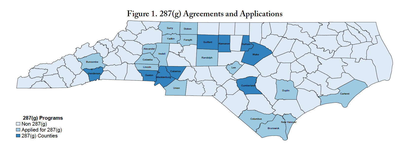
287(g) Participation. We identify 287(g) counties along two margins — program participation and program intensity. Our first indicator of 287(g) adoption is the presence of an active 287(g) MOA, which measures 287(g) participation on the extensive margin. Information on signed 287(g) MOAs is sourced from ICE official records and lists compiled by Nguyen and Gill (2010) and Kostandini et al. (2013). These data include both the date in which the LEA signed a 287(g) MOA and the type of support it authorized — including task forces, jail enforcement, and hybrid programs as mentioned above. Additional data on 287(g) applications and denials were sourced from Pedroza (2019). Figure 1 presents a map of 287(g) program adoptions and applications across the state of North Carolina during our sample horizon. Using population data, we estimate that around 33 percent of North Carolina’s population was covered by 287(g) agreements as of 2010.
6.3 Other Data Demographic Characteristics.
Population and demographic characteristics are sourced from intercensal population estimates from the SEER (Surveillance, Epidemiology, and End Results) Program.9These data are sourced from the NBER website and are published by the National Cancer Institute and the National Institutes of Health. These data provide annual estimates of the resident population at the county level, broken down by age, sex, race, and ethnicity. Using these data we construct measures of the population shares that are Hispanic and non-Hispanic African American. Socioeconomic Conditions. Finally, we collect additional socioeconomic data from the Census Bureau and the Bureau of Labor Statistics (BLS). From the Census Bureau we collect annual estimates of median household income by county from the Small Area Income and Poverty Estimates (SAIPE) program. We also collect data on county unemployment rates from the Local Area Unemployment Statistics (LAUS) files. Since the LAUS data are provided at the monthly level, we compute annual average unemployment rates for our empirical specifications.
7 Results
7.1 Main Results
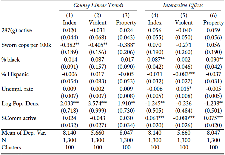
The main results of this paper are shown in Tables 2 and 3. Each table shows OLS estimates for the effect of 287(g) program adoption on the main index crime rates, cost-weighted crime indexes, violent crime rates, and property crime rates. In each specification we regress the natural log of each crime rate per 100,000 or its cost-weighted equivalent on our full set of controls and a set of county and year fixed effects.
Total Crimes. Table 2 presents our main difference-in-differences results for the effects of 287(g) program adoption on county crime rates for the aggregate indexes. The main results are broken down into two main specifications for our dependent variable — the crime rate per 100,000 and and the cost-weighted crime index in line with Mello (2019) and Autor, Palmer, and Pathak (2019). Each dependent variable is expressed as a natural log. Columns 1 through 3 in Table 2 report estimated DD coefficients from (1) of 287(g) program adoption. For each of the main crime indexes, we find small, negative point estimates of around 1.5 to 2 percent — each of which are statistically insignificant and indistinguishable from zero. This is different from the finding of Miles and Cox (2014) who find a statistically significant estimate of around -3 percent for the index crime rate associated with 287(g) adoption. The most predictive variable in our control set for each regression is the natural log of a county’s population density, a common finding in the economics and criminal justice literature. To put these results in terms of the societal cost associated with crime, we rerun Equation (1) and replace each dependent variable with its cost-weighted equivalent in Columns 4 through 6. These specifications allow us the examine whether the 287(g) program was able to create/destroy economic value resulting from fewer/more crimes. Similar to our previous results, we find no empirical evidence to suggest that the adoption of 287(g) policies led to any substantial changes in the average economic costs of crime. Taken together, our baseline findings suggest that 287(g) programs in North Carolina did not have an impact on the main crime rates or the economic costs of crime.
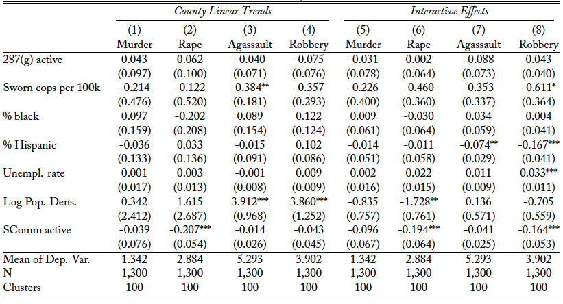
Violent and Property Offenses. Next we examine 287(g) program adoption correlates with changes in the individual index crimes. Since the individual measures of crime tend to be noisier than their aggregates, we only consider the logged crime rates and not their cost-weighted equivalents. These main estimates are shown in Table 3.
First, we examine DD estimates for the breakdown violent crimes in Columns 1 through 4 of Table 3. Stana (2009) notes that a stated goal of the 287(g) program was to aid local law enforcement in the reduction of violent crime committed by violent offenders, therefore a key check of 287(g) program efficacy is to examine violent crime rates. To check whether 287(g) adoption impacted the individual violent crime rates, we rerun (1) with the natural log of each individual violent crime rate as the dependent variable.10To address the issue of zeroes in the murder and rape series, we employ a parametric transformation to approximate the natural log as described in Chalfin and McCrary (2018). Beginning with homicide and rape in Columns 1 and 2, we find positive yet insignificant point estimates of 0.08 and 0.02, respectively. Conversely, we find negative point estimates for the rates of aggravated assault and robbery of around -0.6 and -0.03, although both are similarly insignificant.
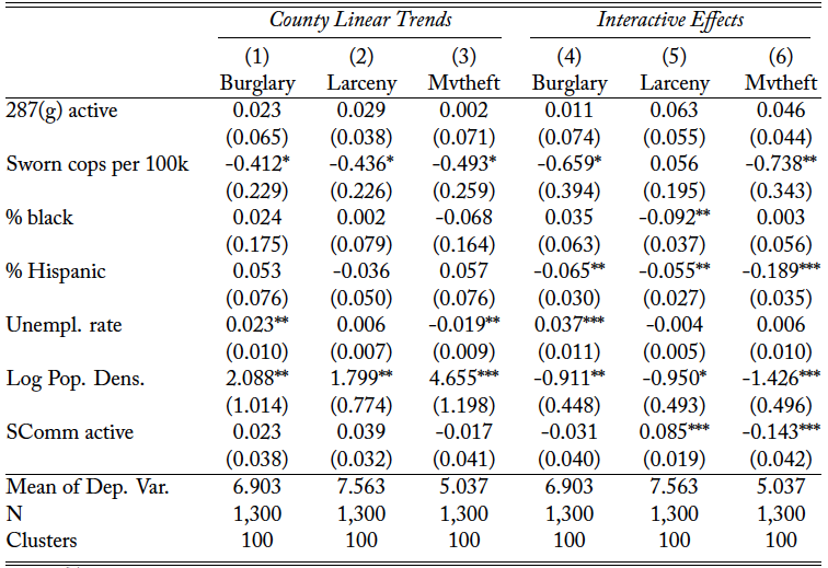
Next, we shift our focus to the main property index crimes in Columns 5 through 7 of Table 3. For the burglary and larceny rates, we find relatively small, negative point estimates of around -0.03 and -0.01, respectively, but each coefficient is statistically indistinguishable from zero. Finally, we find a positive estimate of 0.03 for motor vehicle theft which is, again, statistically insignificant. In each model, we find that the only significant predictor is the log of population density, each carrying a negative coefficient.
Taken together, we find no statistical evidence suggesting that 287(g) programs had an effect on the incidence of the violent or property crime rates. This result holds true under multiple specifications, either expressed as rates per 100,000 or as their cost-weighted equivalents.
7.2 Event Studies
A key assumption underlying our DD research design is that counties that never or have yet to enter 287(g) agreements serve as a valid counterfactual for 287(g) adopters. To test this assumption, we run a series of event-study specifications to compare crime rates between 287(g) and non-287(g) counties in the years prior to and after adoption. Under the parallel trends assumption that counties experienced similar paths in crime rates before entering 287(g) agreements, we would expect the coefficients on leads of the policy variable to be jointly zero.
Results from our event-study specifications are summarized graphically in Figure 2 for the main index crime rates, Figure 3 for the violent crime rates, and Figure 4 for the property crime rates. The associated coefficients are presented in Tables A2, A3, and A4 along with the associated pre-trends tests. For the main index crime rates in Figure 2 we find that the estimated pre-program coefficients fall about the zero line with 95 percent confidence intervals well within the zero mark. Similarly, joint F-tests for significance reveal that we fail to reject the null that the pre-program coefficients are all jointly zero. We find more of the same for most of the individual violent crimes with confidence intervals well within zero. The only exception to this pattern is for homicide, for which we reject the null that all of the pre-treatment coefficients are jointly zero. Further examination of the data show that this rejection results from a main leverage point. In particular, we find that Guilford County’s murder rate was unusually high (at 10.3) in 2003 or 6 years prior to entering a 287(g) program.11For instance, if we run a capped event-study specification that limits pre-trends to 5+ years prior to adoption, we fail to reject that the pre-trends are jointly zero. Finally, this pattern of insignificant pre-program trends persists for each of the individual property crime rates. In nearly every case we fail to reject joint insignificance for pre-trends.
8 Robustness Checks
Before turning to a discussion of our results, we consider a variety of robustness checks. In the previous section, we found no evidence for a connection between 287(g) program and county crime rates following their adoption by local law enforcement. In this section, we discuss various underlying assumptions of our models and conduct tests to verify them. Our first test examines whether our main findings are driven by the presence of unobserved common shocks. We may find that there exists some overarching, unobserved trend in criminal activity that independently affects crime rates and 287(g) adoption. In this case, any relationship we might observe between 287(g) and crime may be spuriously driven by these unobserved factors. We therefore consider two flexible specifications for unobserved common shocks in two forms as described in Section 5 — county-specific linear trends and interactive fixed effects. A second test examines the possibility of geographic spillovers in crime. Consistent with our model of deterrence, if enforcement through the 287(g) program is able to significantly dissuade criminal activity in a home county, we might expect criminal activity to spill over into neighboring counties. It is widely known that the intended targets of 287(g) style enforcement, illegal immigrants, possess high levels of geographic mobility within the U.S. and are highly responsive to increased levels of local immigration enforcement (Amuedo-Dorantes & Lozano, 2019; Bohn, Lofstrom, & Raphael, 2014). We therefore test this hypothesis directly by examining counties that are directly contiguous with 287(g) adopters.
8.1 Testing Specifications
In Table 4 we report estimates for the impact of 287(g) adoption on the main index crime rates using two additional specifications for unobserved common shocks. Since crime rates at the time of 287(g) were falling both nationally and in the State of North Carolina, we may observe a spurious decline in crime among 287(g) counties that tracks overall trends and is unrelated to the effects of the 287(g) program itself. Our first test therefore probes the sensitivity of our estimates to the inclusion of county-specific linear trends. Columns 1 through 3 report difference-in-differences estimates for the main index crime rates that account for county trends. Similar to our baseline results in Table 2, we find insignificant point estimates for each of the main aggregate rates. One key advantage with these specifications is that the inclusion of county trends alleviates concerns of differential trends between 287(g) adopting counties and non-287(g) or yet-to-be-287(g) counties. In the remaining Columns 4 through 6 we introduce an interactive fixed effects estimator described in (4), which provides a more flexible specification for unobserved common shocks than simple linear trends. Comfortingly, results using an interactive effects estimator are numerically similar to estimates using county linear trends and are all statistically indistinguishable from zero.
Moving on to individual violent crime rates, in Table 5 we re-estimate models (3) and (4) for the individual violent crime rates. As in the previous table, we first test the sensitivity of our estimates to the inclusion of county-specific trends. Again, we find a general pattern of statistical insignificance across each of the different violent crime rates. This result is especially interesting for the murder rate, which we found to fail tests for differential pre-287(g) trends. After accounting for county trends, we find that our previous null finding for the effect of 287(g) adoption on the murder rate holds. Moreover, we find that our estimates are similarly insignificant using the interactive effects estimator. Although the existence of differential trends under the canonical two-way fixed effects estimator may confound our estimated effect on homicide rates, we do find that this result holds up under two more flexible specifications for unobserved shocks. We therefore have additional confidence in our null finding of the 287(g) program’s effect on homicide rates.
Finally, estimates shown in Table 6 examine the above model specifications for each of the property crimes. Looking first at Columns 1 through 3, we find that the inclusion of county specific trends has no qualitative effect on our baseline results. In each case, we still find insignificant associations between 287(g) adoption and the main property crime rates. Although the point estimates for burglary and larceny flip sign from negative to positive, the estimated effect of 287(g) remains insignificant. This pattern persists with the inclusion of interactive fixed effects in the remaining columns.
Taken together, our initial difference-in-differences findings are not substantively affected by mis-specification of the unobserved common shocks in our baseline model. Results from our robustness exercises provide more evidence in favor of our initial null results. First, the inclusion of county-specific linear trends allow us to control for potential departures from parallel trends in 287(g) counties versus non-adopters or yet-to adopters. This test therefore provides additional evidence in favor of our main identifying assumption of parallel trends. These results are further bolstered by similar evidence from interactive fixed effect models, which provide a more flexible means to model unobserved shocks and counties’ idiosyncratic responses to them.
8.2 Geographic spillovers
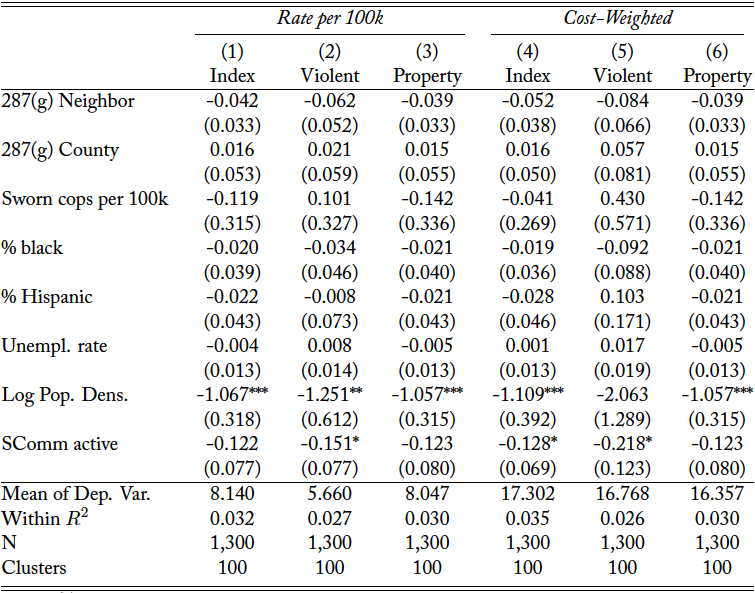
A final test we consider is whether adoption of 287(g) programs led to geographic spillovers in crime rates across county borders. As mentioned above, there is substantial empirical evidence to suggest that immigrants respond to heightened immigration enforcement programs by leaving the area. In the Becker (1968) economic crime model of deterrence, one might expect a similar response from criminal illegal immigrants — leaving their home county in favor of counties with less stringent immigration enforcement attitudes. Holding constant the rate at which criminal immigrants commit offenses, we might therefore expect to see increases in neighboring county crime rates resulting from criminal illegal immigrant exodus from 287(g) adopting counties. We test this hypothesis of geographic spillovers in criminal activity resulting from out-migration by examining crime rates in counties that are directly contiguous to 287(g) counties, before and after their neighbors adopted the policy. To do so, we augment our baseline specification (1) with an indicator variable equal to one for counties in which a neighboring county adopted a 287(g) policy. These two variables therefore allow us to determine whether activation of a nearby 287(g) had an impact on neighboring counties’ average crime rates.
In Table 7 we first consider differences in average crime rates for the main index crime rates, expressed as rates and as cost-weighted indexes. We first examine the estimated coefficients for counties neighboring 287(g) adopters. For each of our estimates coefficients — both for the crime rates per 100,000 and for the cost weighted indexes — we find negative point estimates, each of which are statistically insignificant. Since we cannot reject the null that these coefficients are all zero, we find no empirical evidence to suggest that spillover effects occurred for the major index crime rates. Further, the coefficient estimates associated with actual implementation of 287(g) comport with our prior estimates in terms of statistical significance.
Finally, we examine the possibility for spillover effects for the individual index crime rates. Results for these estimates are presented in Table 8 and they contain slightly different results. Examining our indicator county 287(g) neighboring counties in the first row, we find that two of the coefficient estimates enter statistical significance. Among the violent crimes, we find that the point estimate for robberies is now marginally significant with a negative point estimate of around 10 percent. Similarly, for property crime we find that the neighbor county coefficient is negative and significant for larceny rates at the 5 percent level. This suggests that average larceny rates were around 6 percent lower following the adoption of 287(g) in a neighboring county. This result suggests that, on average, larceny rates fell faster in counties neighboring 287(g) counties than the 287(g) counties themselves. Thus if illegal immigrants move out of 287(g) counties to neighbor counties, there is evidence that they lower the robbery and larceny rates to a statistically significant extent. Besides these two crime rates, we find no subsequent evidence for the existence of spillovers for any other crime rates.
8.3 287(g) Exposure and Crime
While we find no empirical evidence to suggest that the presence of a 287(g) program had an impact on local crime rates, a simple indicator of program presence is less likely to pick up changes in crime rates resulting from heterogeneous intensity of enforcement. Since 287(g) enforcement saw a significant number of noncriminal deportations, we might expect counties with larger noncitizen populations to be impacted differently relative to counties with fewer noncitizens. Specifically, we use data on the noncitizen share from the 2000 Decennial Census to construct measures of sensitivity to 287(g) enforcement. We choose the 2000 Census for two reasons. First, estimates of the noncitizen population are generally unavailable over time for counties. Second, the noncitizen population in 2000 would not incorporate changes in the noncitizen share of the population that may have been removed through 287(g) or the Secure Communities program, which may confound our estimates. To account for this heterogeneity in program effects based on the share of immigrants likely to be affected by 287(g), we consider two additional specifications for our policy variable.
First, we construct an indicator for whether a county is in the top 75th percentile of noncitizen shares in North Carolina and interact it with 287(g) adoption. This specification allows us to examine differences in 287(g)’s effects for counties with large noncitizen populations relative to those that do not. This specification takes the form
(6) 
where  is an indicator for whether county was in the top 75th percentile for the foreign born share as of the 2000 Census. If the 287(g) program impacts crime through deterrence or deportation of criminal illegal immigrants, we would expect a larger effect in counties with more noncitizens. In this case, we would expect the interaction coefficient
  to be negative. As a further test, we consider a more generalized framework that interacts our 287(g) indicator with the noncitizen population share in 2000. This specification allows for intensity of 287(g) enforcement to be continuous proportional to counties’ noncitizen share of the population. This specification takes the form
(7) 
where  is the noncitizen share as of the 2000 Census. The coefficient of interest corresponds to an interaction between 287(g) program adoption and the noncitizen share in 2000. This term measures whether counties with higher noncitizen population shares experienced different effects on crime resulting from the 287(g) program.
Table 9 examines the impact of 287(g) adoption on the main index crime rates while allowing the effect to vary relative to counties’ noncitizen share. Columns 1 through 3 show results from estimating (6) that compare the effects of 287(g) adoption in counties in the top 75th percentile of noncitizens relative to the bottom 75th percentile. For each of our interaction coefficients, we find no evidence that 287(g) had a statistically significant impact on index crime rates in counties with larger noncitizen population shares. We find a similar pattern of insignificance for counties below the 75th percentile for each of the index crime rates. To further probe whether 287(g) adoption affected crime rates for counties with larger noncitizen shares, we consider the generalized framework of (7) in Columns 4 through 6. Similar to our previous results, we find that each of the coefficients are statistically insignificant. This suggests that adopting 287(g) programs did not have an effect on crime that varies according to the share of noncitizens within counties.
Next we examine whether 287(g) had differential effects on the violent index crimes relative to noncitizen population shares. Table 10 reports estimates for the effect of 278(g) adoption on crime rates for each of our interacted policy specifications. First, Columns 1 through 3 show results from interacting 287(g) program adoption with an indicator that a county is at or above the 75th percentile of the noncitizen share. For the individual violent crimes we find insignificant point estimates that are statistically indistinguishable from zero. Moving to Columns 4 through 6, we interact 287(g) adoption with the noncitizen share to determine whether counties with larger noncitizen shares experienced different effects on crime following 287(g) adoption. Again we find statistically insignificant point estimates for the individual violent crime rates.
Finally, we consider our interacted model specifications for the property index crime rates in Table 11. Looking first at Columns 1 through 3, we again find statistically insignificant estimates for 287(g) counties at or above the 75th percentile of the noncitizen share for each of the individual property crime rates. We further find insignificant coefficient estimates for counties adopting 287(g) programs below the 75th percentile of noncitizens. Similarly, results shown in Columns 4 through 6 show no statistically significant evidence for a relationship between 287(g) program adoption and property crime rates relative to a county’s noncitizen share.
Overall, our findings further indicate that there is no significant effects of 287(g) program adoption on crime rates while allowing the program effects to vary according to counties’ noncitizen population share. By allowing the potential effect of 287(g) adoption to vary relative to noncitizen shares, we test the hypothesis that counties with larger shares of noncitizens would be more likely to be impacted by enforcement through 287(g). Further supporting our results in previous sections, we find no empirical evidence to suggest that 287(g) adoption among North Carolina counties impacted crime rates relative to the share of noncitizens it may affect.
9 Discussion
In this paper we examined the staggered implementation of 287(g) programs across counties in the State of North Carolina and the degree to which these programs impacted crime rates. We use a balanced, annual panel of crime data from the FBI to examine whether crime rates were affected by immigration enforcement activity performed by local law enforcement under the 287(g) program. Using a staggered difference-in-differences research design, we find no empirical evidence to suggest that local immigration through the 287(g) program had a noticeable effect on violent and property crime in counties that adopted 287(g) in North Carolina. These results hold for multiple measurements of enforcement, including simple indicators of 287(g) adoption and measures of program intensity, and a series of robustness checks. We further find no evidence for geographic spillovers in crime resulting from the 287(g) program. At best, we find that larceny and robbery rates were likely falling faster in counties neighboring those that entered 287(g) agreements. Altogether, our results are consistent with an evolving literature that finds no sizable effect of immigration enforcement programs and public safety (Miles & Cox, 2014).
Our findings have immediate public policy relevance with the recent reactivation of 287(g) task force agreements by the Trump Administration. Despite its stated objective of pursuing and prioritizing violent criminal offenders for deportation in order to reduce violent crime rates, we find that 287(g) agreements exhibited no effect on crime rates in North Carolina. Under multiple specifications, we find no statistically significant relationship between the adoption or intensity of 287(g) agreements in North Carolina on crime rates. More succinctly, these results demonstrate empirically that the 287(g) program’s objective to reduce crime through the removal of illegal immigrants was not met in the state of North Carolina. Reactivation of the 287(g) program is therefore more likely to impose significant costs to taxpayers than to benefit public safety.
Figures
Figure 1. 287(g) Agreements and Applications
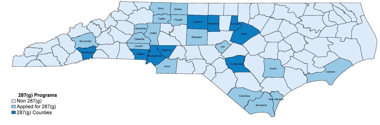
Figure 2. Event-Study Plots, Main Index Offenses
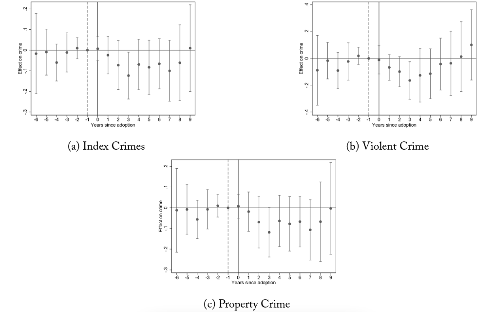
Notes: Figures plot coefficients and confidence intervals on lag and lead policy indicators from DD event-study regressions. The dependent variable in each specification is the natural log of the index crime rate, expressed per 100,000. Each specification includes county and year fixed effects and controls.
Figure 3. Event-Study Plots, Violent Index Offenses
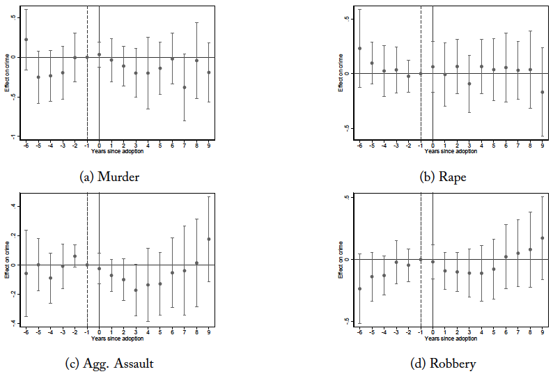
Notes: Figures plot coefficients and confidence intervals on lag and lead policy indicators from DD event-study regressions. The dependent variable in each specification is the natural log of the index crime rate, expressed per 100,000. Each specification includes county and year fixed effects and controls.
Figure 4. Event-Study Plots, Property Index Offenses
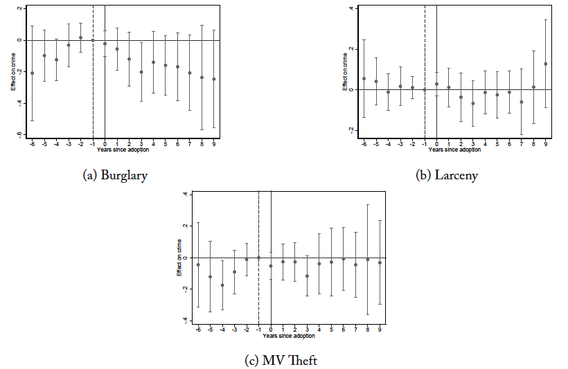
Notes: Figures plot coefficients and confidence intervals on lag and lead policy indicators from DD event-study regressions. The dependent variable in each specification is the natural log of the index crime rate, expressed per 100,000. Each specification includes county and year fixed effects and controls.
Tables
Table 1. Summary Statistics
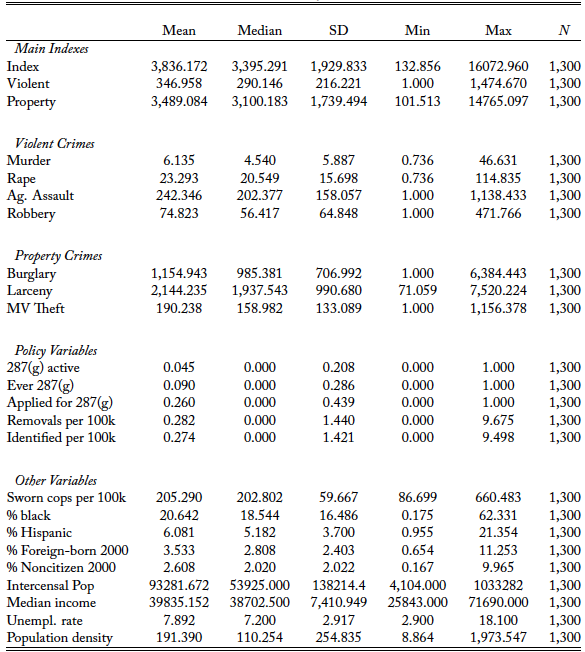
Table 2. Differences in Differences, Main Index Crimes
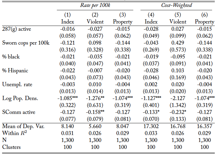
Notes: The dependent variable is the natural log of the index crime rate shown in each column header. 287(g) denotes a dummy variable equal to one in years after adoption of a 287(g) agreement. Each model includes county and year fixed effects and controls for the sworn officer rate per 100,000, % black, % Hispanic, unemployment rate, population density, and Secure Communities activation. Standard errors are clustered by county and significance levels are denoted ∗p < 0.1, ∗ ∗ p < 0.05, ∗ ∗ ∗p < 0.01.
Table 3. Differences in Differences, Individual Crime Rates
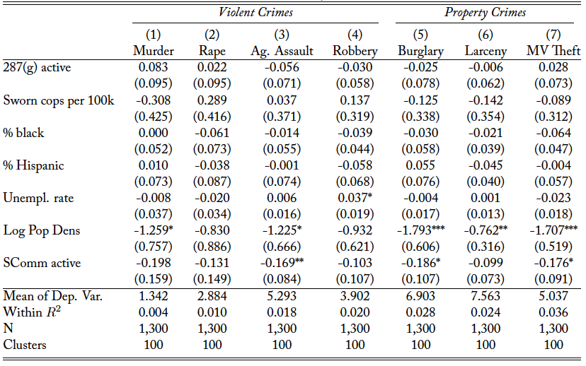
Notes: The dependent variable is the natural log of the index crime rate shown in each column header. 287(g) denotes a dummy variable equal to one in years after adoption of a 287(g) agreement. Each model includes county and year fixed effects and controls for the sworn officer rate per 100,000, % black, % Hispanic, unemployment rate, population density, and Secure Communities activation. Standard errors are clustered by county, and significance levels are denoted ∗p < 0.1, ∗ ∗ p < 0.05, ∗ ∗ ∗p < 0.01.
Table 4. Robustness Checks, Main Index Crime Rates
Notes: The dependent variable is the natural log of the index crime rate shown in each column header. 287(g) denotes a dummy variable equal to one in years after adoption of a 287(g) agreement. Each model includes county fixed effects and controls for the sworn officer rate per 100,000, % black, % Hispanic, unemployment rate, population density, and Secure Communities activation. Columns 1-3 incorporate county-specific linear trends. Columns 4-6 employ the interactive fixed effects estimator of Bai, 2009 with a factor dimension of one. Standard errors are clustered by county and significance levels are denoted ∗p < 0.1, ∗ ∗ p < 0.05, ∗ ∗ ∗p < 0.01.
Table 5. Robustness Checks, Violent Crime Rates
Notes: The dependent variable is the natural log of the index crime rate shown in each column header. 287(g) denotes a dummy variable equal to one in years after adoption of a 287(g) agreement. Each model includes county fixed effects and controls for the sworn officer rate per 100,000, % black, % Hispanic, unemployment rate, population density, and Secure Communities activation. Columns 1-3 incorporate county-specific linear trends. Columns 4-6 employ the interactive fixed effects estimator of Bai, 2009 with a factor dimension of one. Standard errors are clustered by county and significance levels are denoted ∗p < 0.1, ∗ ∗ p < 0.05, ∗ ∗ ∗p < 0.01.
Table 6. Robustness Checks, Property Crime Rates
Notes: The dependent variable is the natural log of the index crime rate shown in each column header. 287(g) denotes a dummy variable equal to one in years after adoption of a 287(g) agreement. Each model includes county fixed effects and controls for the sworn officer rate per 100,000, % black, % Hispanic, unemployment rate, population density, and Secure Communities activation. Columns 1-3 incorporate county-specific linear trends. Columns 4-6 employ the interactive fixed effects estimator of Bai, 2009 with a factor dimension of one. Standard errors are clustered by county and significance levels are denoted ∗p < 0.1, ∗ ∗ p < 0.05, ∗ ∗ ∗p < 0.01.
Table 7. Geographic Spillovers, Main Index Crime
Notes: The dependent variable is the natural log of the index crime rate shown in each column header. 287(g) denotes a dummy variable equal to one in years after adoption of a 287(g) agreement. Each model includes county and year fixed effects and controls for the sworn officer rate per 100,000, % black, % Hispanic, unemployment rate, population density, and Secure Communities activation. Standard errors are clustered by county and significance levels are denoted ∗p < 0.1, ∗ ∗ p < 0.05, ∗ ∗ ∗p < 0.01.
Table 8. Geographic Spillovers, Individual Crime Rates
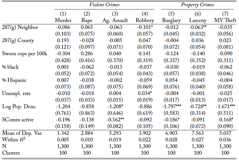
Notes: The dependent variable is the natural log of the index crime rate shown in each column header. 287(g) denotes a dummy variable equal to one in years after adoption of a 287(g) agreement. Each model includes county and year fixed effects and controls for the sworn officer rate per 100,000, % black, % Hispanic, unemployment rate, population density, and Secure Communities activation. Standard errors are clustered by county and significance levels are denoted ∗p < 0.1, ∗ ∗ p < 0.05, ∗ ∗ ∗p < 0.01.
Table 9. Impact of 287(g) Programs on Crime, Alternate Measures
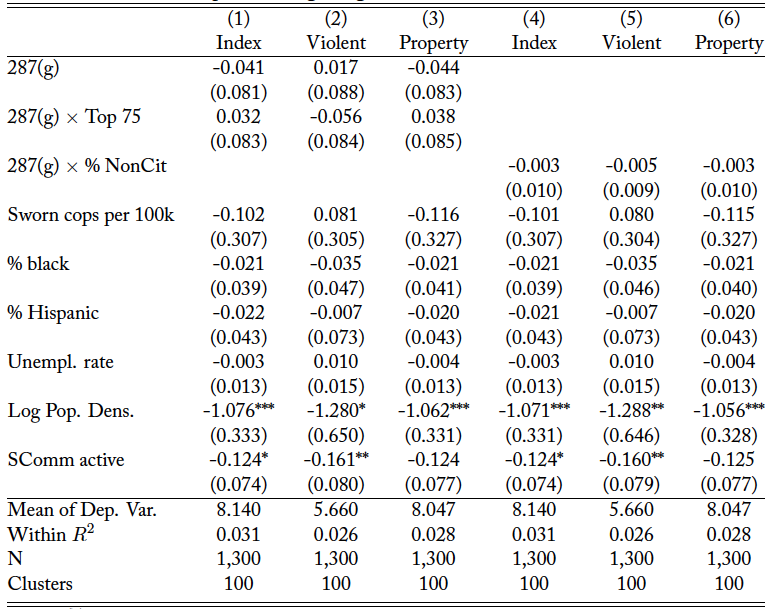
Notes: The dependent variable is the natural log of the index crime rate shown in each column header. 287(g) denotes a dummy variable equal to one in years after adoption of a 287(g) agreement. Top 75 denotes counties in the top 75th percentile of the noncitizen share as of the 2000 Census. % NonCit denotes the share of noncitizens as of the 2000 Census. Each model includes county and year fixed effects and controls for the sworn officer rate per 100,000, % black, % Hispanic, unemployment rate, population density, and Secure Communities activation. Standard errors are clustered by county and significance levels are denoted ∗p < 0.1, ∗ ∗ p < 0.05, ∗ ∗ ∗p < 0.01.
Table 10. Impact of 287(g) Programs on Violent Crime, Alternate Measures
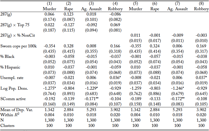
Notes: The dependent variable is the natural log of the index crime rate shown in each column header. 287(g) denotes a dummy variable equal to one in years after adoption of a 287(g) agreement. Top 75 denotes counties in the top 75th percentile of the noncitizen share as of the 2000 Census. % NonCit denotes the share of noncitizens as of the 2000 Census. Each model includes county and year fixed effects and controls for the sworn officer rate per 100,000, % black, % Hispanic, unemployment rate, population density, and Secure Communities activation. Standard errors are clustered by county and significance levels are denoted ∗p < 0.1, ∗ ∗ p < 0.05, ∗ ∗ ∗p < 0.01.
Table 11. Impact of 287(g) Programs on Crime, Alternate Measures
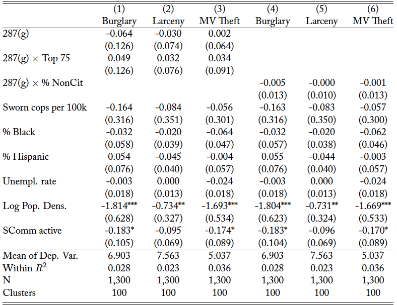
Notes: The dependent variable is the natural log of the index crime rate shown in each column header. 287(g) denotes a dummy variable equal to one in years after adoption of a 287(g) agreement. Top 75 denotes counties in the top 75th percentile of the noncitizen share as of the 2000 Census. % NonCit denotes the share of noncitizens as of the 2000 Census. Each model includes county and year fixed effects and controls for the sworn officer rate per 100,000, % black, % Hispanic, unemployment rate, population density, and Secure Communities activation. Standard errors are clustered by county and significance levels are denoted ∗p < 0.1, ∗ ∗ p < 0.05, ∗ ∗ ∗p < 0.01.
Data Appendix
A Data Sources and Variable Definitions
A.1 Data Sources
Crime Data: Our primary source for crime data is the Uniform Crime Reports (UCR) published by the FBI. The UCR data represent the main source of crime data in the United States. Data on reported crimes are taken from the Return A file, which records offenses known to law enforcement. Through the UCR program, individual law enforcement agencies (LEAs) submit monthly reports on “index crimes” and “breakdown offenses” to the FBI. The main index crimes are broken down into violent crimes (homicide, forcible rape, robbery, and aggravated assault) and property crimes (burglary, larceny over $50, and motor vehicle theft).12The data also include simple assault, which is not an index crime. Agencies also report breakdown offenses, which represent subcategories to the main index offenses, such as manslaughter, various types of thefts, etc. In our subsequent cleaning procedures, we consider only the main index offenses.
Police Employment: We collect data on police employment at the agency level from the FBI Police Employment files. These data are similarly collected through the UCR program on an annual basis and list the number of full-time sworn police officers and civilian employees for each agency that reports through the UCR as of October 31st in a given year (Chalfin & McCrary, 2018). These data also include monthly Law Enforcement Officers Killed and Assaulted (LEOKA) reports, which enumerate the number of assaults against police officers and the number of officers killed by accidental or felonious actions.
Population: Population data are from the National Institutes of Health SEER (Surveillance, Epidemiology, and End Results) Program. The SEER Program produces annual, county-level intercensal estimates of the resident population based on data from the Census Bureau. These data are further broken down by age, sex, race, and ethnicity. We source these data from the NBER, which provides cleaned versions of the data on their website.
Unemployment: Unemployment data come from the Local Area Unemployment Statistics (LAUS) files produced by the Bureau of Labor Statistics. The LAUS files provide estimates of the labor force, employment, and unemployment by year on a monthly basis for counties. Using the monthly data, we compute annual averages for each county.
Poverty and Income: Data on poverty rates and income are sourced from the Census Bureau’s Small Area Income and Poverty Estimates (SAIPE) program. The SAIPE program draws on multiple administrative datasets to produce annual modeled estimates of median household income and poverty rates for states and counties. To produce these data, the SAIPE program uses multiple regression and shrinkage methods. These data provide estimates of the population share of all ages in poverty and median household income.
Geography: We draw on geographic data by county from the 2010 Gazetteer files from the Census Bureau. The Gazetteer files contain information on counties’ land and water area in miles and kilometers and their latitude and longitude coordinates.
A.2 Variable Descriptions
Log crime per 100k: The log crime rate per 100,000 residents for each index crime. The violent crime index is the sum of homicide, forcible rape, robbery, and aggravated assault. The property index is the sum of burglary, larceny over $50, and motor vehicle theft. The population denominator is from the SEER annual population estimates.
Log crime Cost: The log cost of crime using the estimated social cost of violent crime ($ 67,794) and property crime ($ 4,064).
Log cops per 100k: The natural log of the sworn officer rate per 100,000 residents. This variable is lagged by one year in line with the literature, since police employment data is collected late in the year as of October 31st. The population denominator is from the SEER annual population estimates.
287(g) active: An indicator variable equal to one if the county has an active 287(g) agreement with ICE.
% black: The share of black residents who do not identify as Hispanic.
% Hispanic: The share of Hispanic residents who identify as an race.
Unemployment rate: The number of unemployed workers as a share of the total county labor force.
Log population density: The log population divided by land area in square miles.
SComm active: An indicator variable equal to one if the Secure Communities program is active in the county.
287(g) neighbor: An indicator variable equal to one following the adoption of a 287(g) agreement in a directly contiguous county.
Noncitizen: Population share of noncitizens from the 2000 Decennial Census.
Top 75: Top 75th percentile of noncitizen share from the 2000 Decennial Census.
B Additional Tables
Table A1. 287(g) Agreements in North Carolina
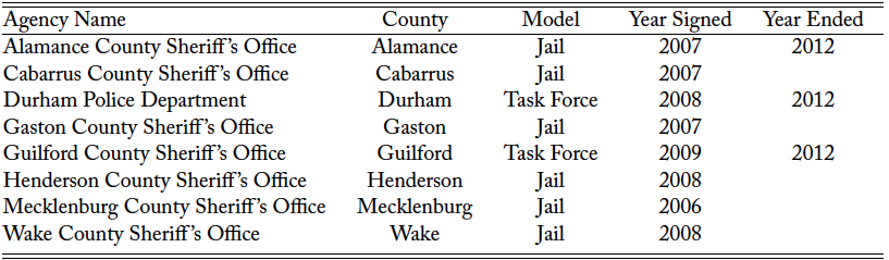
Notes: Table identifies 287(g) programs in North Carolina by agency and lists the year in which they were signed and terminated, where applicable. All 287(g) task force agreements were terminated nationally in 2012.
Table A2. Event-Study Estimates, Main Index Crime Rates
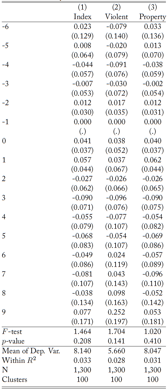
Notes: ∗p < 0.1, ∗ ∗ p < 0.05, ∗ ∗ ∗p < 0.01.
Table A3. Event-Study Estimates, Violent Crime Rates
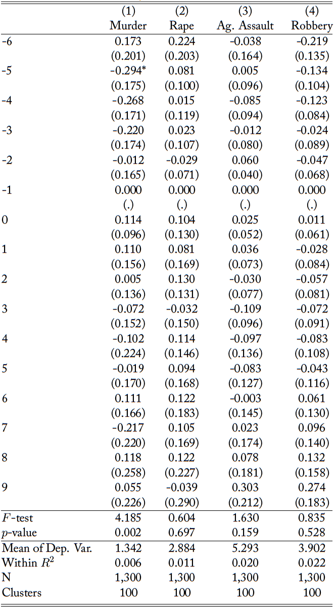
Notes: ∗p < 0.1, ∗ ∗ p < 0.05, ∗ ∗ ∗p < 0.01.
Table A4. Event-Study Estimates, Property Crime Rates
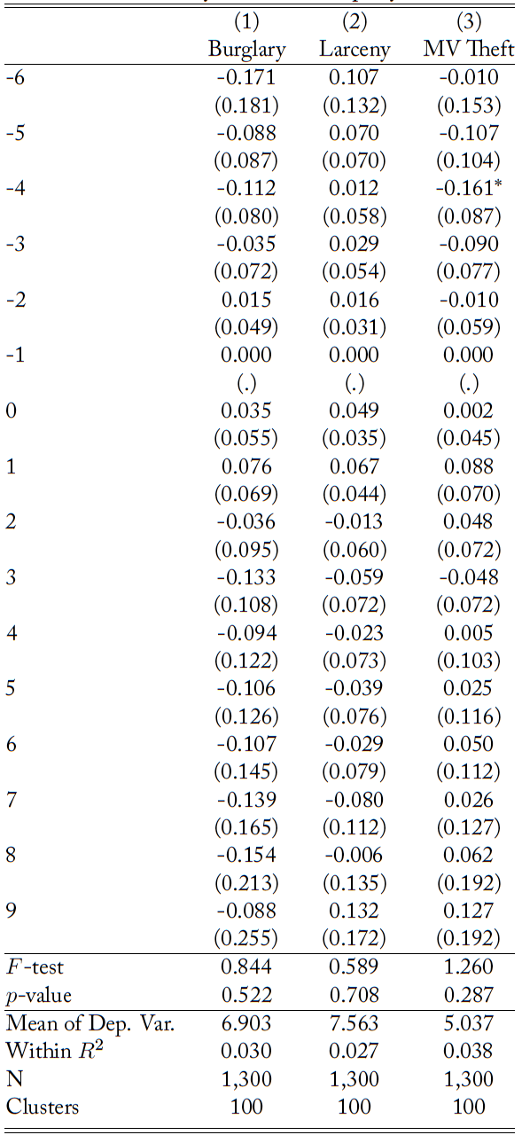
Notes: ∗p < 0.1, ∗ ∗ p < 0.05, ∗ ∗ ∗p < 0.01.
References
Amuedo-Dorantes, C., & Lozano, F. A. (2019). Interstate Mobility Patterns of Likely Unauthorized Immigrants: Evidence from Arizona. Journal of Economics, Race, and Policy, 2(1), 109–120.
Autor, D. H., Palmer, C. J., & Pathak, P. A. (2019). Ending Rent Control Reduced Crime in Cambridge.
AEA Papers and Proceedings, 109, 381–384.
Bai, J. (2009). Panel Data Models With Interactive Fixed Effects. Econometrica, 77(4), 1229–1279. Becker, G. S. (1968). Crime and Punishment: An Economic Approach. Journal of Political Economy, 76(2), 169–217.
Bertrand, M., Duflo, E., & Mullainathan, S. (2004). How Much Should We Trust Differences-In-Differences Estimates? Quarterly Journal of Economics, 119(1), 249–275.
Bohn, S., Lofstrom, M., & Raphael, S. (2014). Did the 2007 Legal Arizona Workers Act Reduce the State’s Unauthorized Immigrant Population? Review of Economics and Statistics, 96(2), 258–269.
Bohn, S., & Santillano, R. (2017). Local Immigration Enforcement and Local Economies. Industrial Relations: A Journal of Economy and Society, 56(2), 236–262.
Bove, V., & Gavrilova, E. (2017). Police Officer on the Frontline or a Soldier? The Effect of Police Militarization on Crime. American Economic Journal: Economic Policy, 9(3), 1–18.
Chalfin, A., & McCrary, J. (2018). Are U.S. Cities Underpoliced? Theory and Evidence. Review of Economics and Statistics, 100(1), 167–186.
Cohen, M. A., & Piquero, A. R. (2009). New Evidence on the Monetary Value of Saving a High Risk Youth. Journal of Quantitative Criminology, 25(1), 25–49.
Cox, A. B., & Miles, T. J. (2013). Policing Immigration. University of Chicago Law Review, 80(1), 87–136. Retrieved from https://chicagounbound.uchicago.edu/uclrev/vol80/iss1/5/.
Cox, A. B., & Posner, E. A. (2012). Delegation in Immigration Law. University of Chicago Law Review, 79(4), 1285–1349. Retrieved from https://lawreview.uchicago.edu/publication/delegation-immigration-law.
Dee, T. S., & Murphy, M. (2019). Vanished Classmates: The Effects of Local Immigration Enforcement on School Enrollment. American Educational Research Journal.
FBI. (2013). Summary Reporting System (SRS) User Manual . Uniform Crime Reporting (UCR) Program. Retrieved from https://www.fbi.gov/file-repository/ucr/ucr-srs-user-manual-v1.pdf/view.
Gobillon, L., & Magnac, T. (2016). Regional Policy Evaluation: Interactive Fixed Effects and Synthetic Controls. Review of Economics and Statistics, 98(3), 535–551.
Green, D. (2016). The Trump Hypothesis: Testing Immigrant Populations as a Determinant of Violent and Drug-Related Crime in the United States. Social Science Quarterly, 97(3), 506–524.
Harris, M. C., Park, J., Bruce, D. J., & Murray, M. N. (2017). Peacekeeping Force: Effects of Providing Tactical Equipment to Local Law Enforcement. American Economic Journal: Economic Policy, 9(3).
Hines, A. L., & Peri, G. (2019). Immigrants’ Deportations, Local Crime and Police Effectiveness (DP No. 12413). IZA Institute of Labor Economics. Retrieved from https://www.iza.org/publications/dp/12413/immigrants-deportations-local-crime-and-police-effectiveness.
ICE. (n.d.-a). Delegation of Immigration Authority Section 287(g) Immigration and Nationality Act Factsheet. Washington DC: U.S. Immigration and Customs Enforcement. Accessed: August 11, 2017. Retrieved from https://www.ice.gov/287g.
ICE. (n.d.-b). Secure Communities Fact Sheet. Washington DC: U.S. Department of Homeland Security. Accessed: August 14, 2017. Retrieved from https://www.ice.gov/secure-communities.
ICE. (2009). Secure Communities: Quarterly Report. Washington DC: First Quarter FY2009 Report to Congress, Department of Homeland Security. Retrieved from https://www.ice.gov/doclib/foia/secure_communities/congressionalstatusreportfy091stquarter.pdf ICE. (2010). 287(g) Master Stats – Oct. 31, 2010. Washington DC: U.S. Department of Homeland Security, FOIA. Retrieved from http://www.ice.gov/doclib/foia/reports/287g-masterstats2010oct31.pdf.
Ifft, J., & Jodlowski, M. (2016). Is ICE Freezing US Agriculture? The Impact of Local Immigration Enforcement on Farm Profitability and Structure (Annual Meeting, Boston, Massachusetts No. 235950). Agricultural and Applied Economics Association. Retrieved from https://EconPapers.repec.org/RePEc:ags:aaea16:235950.
Kandel, W. A. (2016). Interior Immigration Enforcement: Criminal Alien Programs. Retrieved from https://fas.org/sgp/crs/homesec/R44627.pdf.
Kostandini, G., Mykerezi, E., & Escalante, C. (2013). The Impact of Immigration Enforcement on the U.S. Farming Sector. American Journal of Agricultural Economics, 96(1), 172–192.
Maltz, M. D., & Targonski, J. (2002). A Note on the Use of County-Level UCR Data. Journal of Quantitative Criminology, 18(3), 297–318.
Maltz, M. D., & Weiss, H. E. (2006). Creating a UCR Utility. Final Report to the National Institute of Justice.
Mears, D. P. (2001). The Immigration-Crime Nexus: Toward an Analytic Framework for Assessing and Guiding Theory, Research, and Policy. Sociological Perspectives, 44(1), 1–19.
Mello, S. (2019). More COPS, Less Crime. Journal of Public Economics, 172, 174–200.
Miles, T. J., & Cox, A. B. (2014). Does Immigration Enforcement Reduce Crime? Evidence from Secure Communities. Journal of Law and Economics, 57(4), 937–973.
Nguyen, M. T., & Gill, H. (2010). The 287(g) Program: The Costs and Consequences of Local Immigration Enforcement in North Carolina Communities. Chapel Hill: The Latino Migration Project, The Institute for the Study of the Americas, The University of North Carolina at Chapel Hill.
Nguyen, M. T., & Gill, H. (2016). Interior Immigration Enforcement: The Impacts of Expanding Local Law Enforcement Authority. Urban Studies, 53(2), 302–323.
Outten-Mills, D. L. (2012). The Performance of 287(g) Agreements FY 2012 Follow-Up. Washington DC: Department of Homeland Security, Office of the Inspector General. Retrieved from https://www.hsdl.org/?view&did=723724
Pedroza, J. (2019). Where Immigration Enforcement Agreements Stalled: The Location of Local 287(g) Program Applications and Inquiries (2005-2012). Working Paper.
Pham, H., & Van, P. H. (2010). The Economic Impact of Subfederal Immigration Regulation: An Empirical Analysis. Cardozo Law Review, 32(2), 485–518.
Rhodes, S. D., Mann, L., Simán, F. M., Song, E., Alonzo, J., Downs, M., … Hall, M. A. (2015). The Impact of Local Immigration Enforcement Policies on the Health of Immigrant Hispanics/Latinos in the United States. American Journal of Public Health, 105(2), 329–337.
Rosenblum, M. R., & Kandel, W. A. (2013). Interior Immigration Enforcement Prior to 2014: Programs Targeting Criminal Aliens (CRS Report No. R42057). Retrieved from https://www.hsdl.org/?view&did=744667.
Rugh, J. S., & Hall, M. (2016). Deporting the American Dream: Immigration Enforcement and Latino Foreclosures. Sociological Science, 3(46), 1053–1076.
Stana, R. A. (2009). Immigration Enforcement: Better Controls Needed over Program Authorizing State and Local Enforcement of Federal Immigration Laws (GAO-09-109). Washington DC: Government Accountability Office. Retrieved from https://www.gao.gov/products/GAO-09-109.
Totty, E. (2017). The Effect of Minimum Wages on Employment: A Factor Model Approach. Economic Inquiry, 55(4), 1712–1737.
United States Cong. House. Committee on Government Reform, Subcommittee on Criminal Justice, Drug Policy, and Human Resources. (2006). Empowering Local Law Enforcement to Combat Illegal Immigration. Hearings, August 25, 2006. Washington DC: House Hearing, 109th Cong. 2nd sess. Government Printing Office. Retrieved from https://www.govinfo.gov/content/pkg/CHRG-109hhrg36029/html/CHRG-109hhrg36029.htm United States Cong. House. Committee on Homeland Security. (2009). Examining 287(g): The Role of State and Local Law Enforcement in Immigration Law. Hearings, March 4, 2009.
Washington DC: House Hearing, 111th Cong. 1st sess. Government Printing Office. Retrieved from https://www.govinfo.gov/content/pkg/CHRG-111hhrg49374/html/CHRG-111hhrg49374.htm United States v. Johnson. (2012). 1:12-cv-1349 (M.D.N.C.) Retrieved from https://www.courtlistener.com/docket/5071512/united-states-v-johnson/.
Weissman, Deborah M and Headen, Rebecca C. and Parker, Katherine Lewis. (2009). The Policies and Politics of Local Immigration Enforcement Laws: 287(g) Program in North Carolina. American Civil Liberties Union of North Carolina Legal Foundation and Immigration and Human Rights Policy Clinic at the University of North Carolina at Chapel Hill.